Resource Distribution Curve Analysis

Introduction

xerPlanner’s resource distribution curve analysis reviews how labor hours are distributed over time, considering both work already performed and work remaining to be executed. Its purpose is to identify abnormal workload patterns that may reveal planning issues, operational continuity problems, or schedule feasibility risks.

Unlike aggregated indicators such as Earned Value, this analysis does not summarize performance into a single number. Its value lies in showing the time-based shape of the effort: when hours are concentrated, whether there are peaks that may be difficult to sustain, whether work is loaded toward the end, whether there are empty periods, or whether there is an excessive gap between early and late curves.

In real projects, these patterns can say a lot about the quality of the plan.

What the analysis shows

xerPlanner generates distribution curves for labor resources. The analysis is presented at two levels:

• a consolidated curve in the main body of the report, grouping all project labor resources;
• individual curves in the appendices, where the same analysis is replicated for each labor resource.

This separation is important because a consolidated curve may look reasonable while still hiding issues in specific resources. For example, the project total may appear balanced, while one discipline has an excessive peak, another is heavily loaded toward the end, and another has long periods with almost no workload.

The consolidated curve provides a global view. The individual curves help identify where the issues come from.

How to read the chart

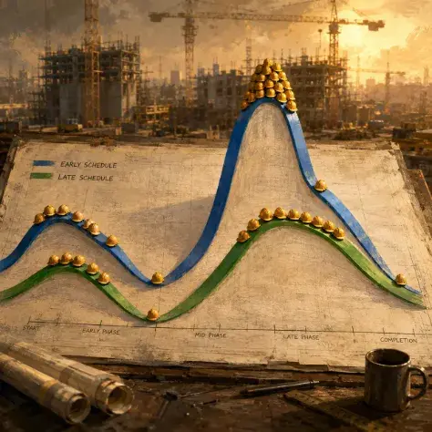
Each chart combines a histogram of hours by period with cumulative curves overlaid on the same visual. The horizontal axis represents time, and the vertical axis represents labor hours distributed in each period.

The information is organized around the Data Date, which separates actual work already performed from remaining work.

Before the Data Date, the chart shows actual hours. After the Data Date, it shows the projected distribution of remaining work from two perspectives:

• early remaining, calculated using the schedule’s early dates;
• late remaining, calculated using the schedule’s late dates.

Displaying both remaining curves in the same chart makes it possible to observe the available range of flexibility. If the early and late curves are close together, the movement margin is limited. If they are far apart, there is more float, although an excessive gap may also reveal weak logic or poorly integrated activities.

The chart timescale is automatically adjusted based on the total project duration to keep the visual readable:

• projects up to 11 months: weekly scale;
• projects from 1 to 3 years: monthly scale;
• projects longer than 3 years: quarterly scale.

If the project has not started yet, the chart shows only remaining work. If it has already finished, it shows only actual hours. In projects in progress, both sections coexist, separated by the Data Date.

Effort peak

The first aspect analyzed by xerPlanner is the effort peak, meaning the period with the highest concentration of labor hours.

A moderate peak may be normal. Many projects have periods of higher intensity, especially during construction, installation, commissioning, or partial turnover phases. The issue appears when one period concentrates a much higher number of hours than the rest of the distribution.

An excessive peak may indicate that the schedule assumes a resource mobilization that is difficult to sustain, that many activities were scheduled in parallel without considering real availability constraints, or that the logic concentrates too much work into a very narrow window.

In these cases, the finish date may look achievable in the schedule, but it may depend on an unrealistic operational condition.

Remaining work skew

The second aspect is the remaining work skew, meaning how the pending workload is distributed between the Data Date and the project finish.

A cumulative curve that rises quickly at the beginning and then flattens indicates that most remaining work is loaded into the early periods. In general, this is favorable because it leaves more margin at the end to absorb contingencies.

By contrast, a curve that progresses slowly at the beginning and becomes steeper toward the end indicates that the schedule concentrates too much work in the final periods. This can be risky because it reduces the ability to react to delays, interferences, access restrictions, or lower productivity.

A schedule with too much work loaded at the end may look feasible in terms of dates, but fragile from an operational perspective.

Gap between early and late remaining work

The third aspect is the gap between the cumulative early remaining curve and the cumulative late remaining curve.

This difference visually represents the float available for activities with assigned resources. A moderate gap is normal and even desirable because it indicates that the schedule has some flexibility.

However, an excessive gap can be a warning sign. It may indicate that many activities have too much freedom of movement, that the logic network is weakly connected, or that the schedule is not sufficiently constraining the execution sequence.

This matters because overly flexible logic may make projected dates look less committed than they really are. It may also make risk analysis more difficult, because the model relies on a network that does not necessarily represent a sufficiently controlled sequence.

Valleys in the distribution

The fourth aspect is the identification of valleys, meaning periods where the workload drops significantly compared with nearby periods and then rises again.

These valleys may represent discontinuities in resource utilization. In practice, they may imply that part of the team is left without work for a period and then must be mobilized again later.

This is not always an error. There may be valid reasons for a temporary workload reduction, such as waiting windows, planned interferences, access restrictions, or phase transitions. But when valleys are not justified, they may reveal problems in the logic sequence or in resource planning.

In real projects, these discontinuities may have important costs: demobilization, loss of learning curve, later hiring, risk of key personnel not being available when needed, and reduced operational continuity.

Why this analysis adds value

The time-based distribution of resources is often reviewed late or only superficially. A schedule may show correct dates while still requiring an amount of labor that is impossible to sustain in certain periods.

This analysis helps detect that type of issue before it becomes an execution problem. It is not enough to know that the work fits within the available time; it also matters whether the resource load required to meet that time frame is reasonable.

Resource distribution curve analysis is especially useful in three moments:

• during bid schedule review, to assess whether the contractor’s proposal is feasible;
• during periodic project control, to detect resource planning issues early;
• during forensic or retrospective analysis, to understand whether certain execution problems were already embedded in a poor workload distribution.

In this sense, xerPlanner does not only review schedule logic. It also helps determine whether the planned effort has a reasonable shape over time.

Conclusion

A well-built schedule should not only indicate when activities are executed. It should also show a resource distribution that is coherent, sustainable, and compatible with the project’s operational reality.

Resource distribution curve analysis helps identify excessive peaks, work loaded toward the end, wide gaps between early and late dates, and valleys that may affect team continuity. These patterns do not always represent errors, but they are signals that should be reviewed.

In complex projects, a resource curve can reveal issues that are not clearly visible in an activity table or in an aggregated indicator. Reviewing this distribution helps improve schedule quality, anticipate execution risks, and strengthen the team’s ability to technically defend its plan.